Running the imaging pipeline¶

This recipe explains how to run the imaging pipeline. The imaging pipeline is used to create images, in standard FITS format, from LOFAR TBB data.

Beamforming¶

The imaging pipeline and its principal component the imager uses the technique of beamforming to calculate the intensity of each pixel in the final image.

The essence of beam forming is to add the signals from different antennas in order to achieve sensitivity to one direction. This direction is determined by time shifts of the signals from the antennas. Although beam forming is used for all kinds of signals it is easily depicted with radio pulses. As an example figure shows the geometry of the source and two antennas. A pulse originating at the source will first arrive at antenna 2 and then at antenna 1. To have the pulse at the same position in both datasets the dataset of antenna 1 has to be shifted in relation to the one from antenna 2 by the delay that corresponds to the distance from antenna 1 to point A. If both datasets are then added up, the pulse will be enhanced in the resulting data, while a pulse from another direction will be smeared out. The same is true for continuous signals from a source. If one chooses not antenna2 but a point in between the antennas as the reference position, then the data from both antennas has to be shifted (e.g. antenna 1 by the delay ant. 1 to point B and antenna 2 by ant. 2 to point C in the figure). To calculate the geometric delays we first transform the antenna positions into the coordinate system aligned to the direction of the source:

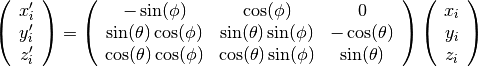
$\left(\begin{array}{c} x_{i}'\\ y_{i}'\\ z_{i}'\end{array}\right) = \left(\begin{array}{ccc} -\sin(\phi) & \cos(\phi) & 0 \\ \sin(\theta)\cos(\phi) & \sin(\theta)\sin(\phi) & -\cos(\theta) \\ \cos(\theta)\cos(\phi) & \cos(\theta)\sin(\phi) & \sin(\theta)\end{array}\right) \left(\begin{array}{c}x_{i} \\ y_{i} \\ z_{i}\end{array}\right)$

Here $x_{i}, y_{i}, z_{i}$ are the antenna positions relative to a reference position; $\phi$ is the azimuth angle and $\theta$ the elevation of the given direction; $x_{i}', y_{i}', z_{i}'$ are the antenna positions in the source coordinate system, whose z-axis points in the direction of the source.

If the incoming signal is a plane wave (i.e. the source is far away) then the relative distance is $z_{i}'$ and the delay is $z_{i}'/c$ . If the signal is a spherical wave with a radius of curvature of $R_{\mathrm{curv}}$ (i.e. a signal like that from a point source at $(0,0,R_{\mathrm{curv}})$ in source coordinates), then the relative distances are:

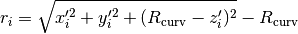
$r_{i} = \sqrt{x_{i}'^{2} + y_{i}'^{2} + (R_{\mathrm{curv}} - z_{i}')^{2}} - R_{\mathrm{curv}}$

With the delays being $r_{i}/c$ . To efficiently do shifts by sub-sample steps, the shift itself is done by Fourier transforming the time domain data to the frequency space and then multiplying a phase gradient to the data. Adding the data from all antennas together and squaring the result directly gives the spectral power distribution for this pixel:

$P(\vec{\rho})[\omega] = \left|S(\vec{\rho})[\omega]\right|^{2} = \left|\sum_{i=1}^{N_{\mathrm{ant}}}w_{i}(\vec{\rho})[\omega]s_{i}[\omega]\right|^{2}$

With $P(\vec{\rho})$ being the power in the direction $\vec{\rho}$ , $S(\vec{\rho})$ the beam formed data, $N_{\mathrm{ant}}$ the number of antennas, $w_{i}(\vec{\rho})[\omega] = e^{i\omega r_{i}/c}$ the weighting factor of the phase gradient and $s_{i}[\omega]$ the frequency domain data of the single antennas.